Here, let’s take a detailed look at creating and using a Pivot table in Google Sheets. Content
What is Google Sheets Pivot Table
While normal tables are ideal for handling large amounts of data, it is quite difficult to analyze or get meaningful information from them. Google Sheets pivot tables come in handy as they can summarize massive amounts of data on any rows/columns in a spreadsheet. For example, a Google Sheets pivot table can be used by a business owner to analyze which store has made maximum sales revenue for a specific month. In general, a pivot table in Google Sheets can be used to calculate averages, sums, or any other statistics from a large data set.
How to Create a Pivot Table in Google Sheets
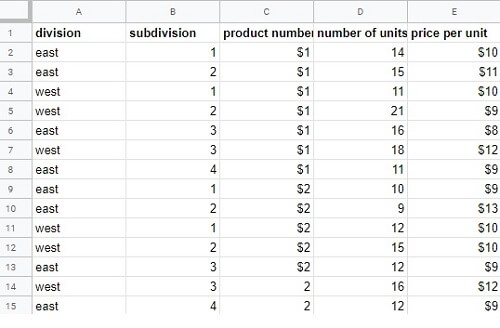
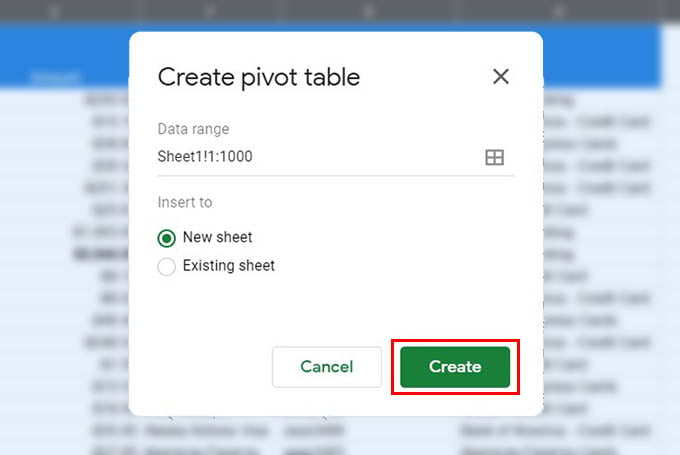
Let’s see how to create a Pivot table in Google Sheets from your existing table or large data set. For example, let’s take a simple data set that has the sales information from various divisions of the company for a specific month. Before starting to create a pivot table, you need to make sure that every column is associated with a header/title. Now, let’s see how to get meaningful information out of this data set using the Pivot table in Google Sheets we just created.
How to Edit a Google Sheets Pivot Table
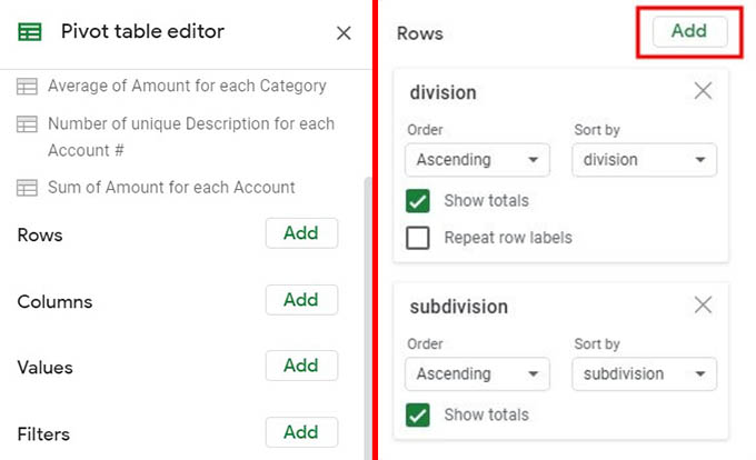
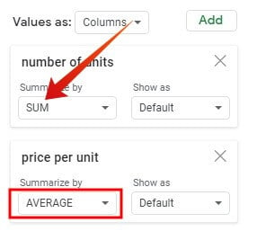
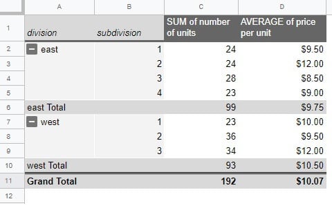
After creating a new pivot table in Google Sheets, you can sort and find out the information you want from the data. Let’s take the sample data set mentioned above. Here, we will find out the total number of units sold by every division and the average price per unit using the Google Sheets pivot table data. Likewise, you can use other formulas like MAX, MIN, AVERAGE, MEDIAN and more.
How to Customize a Pivot Table in Google Sheets
Google sheets provide a lot of options to customize the pivot table. Let’s take a brief look at some of the most commonly used options:
Sort Rows or Columns in Pivot Table
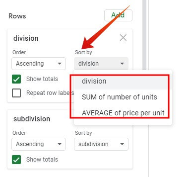
You can sort the Google Sheets pivot table data by values, row, or column names. In the Pivot table editor window, you will find the “Sort by” drop-down box which lists the names of all rows and columns of your pivot table. Based on your need, you can sort the column or row based on your requirement.
Show Value as Percentage
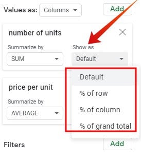
By default, values (eg. SUM of the number of units) will be displayed as numbers. However, if you would like to display them as a percentage by comparison with whole data, then you can do that as well. Just click the Pivot table. Under Values, click the drop-down box titled Show as and select any of the options given below:
% of row% of column% of grand total
By default, the drop-down box is set to “Default“. You can choose aby of the options to show the pivot table in different formats.
Grouping Data in Google Sheets Pivot Table
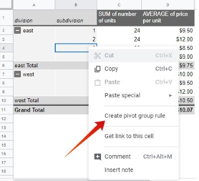
You can select a set of values from the pivot table in Google Sheets and group them together based on a rule or manually. To manually create a Google Sheets pivot group, select all the cells you want to group and right-click the cells. Then, select the Create Pivot group. In order to group rows by rule, right-click a cell and select Create Pivot group rule. Then, you will see a small window titled Grouping rule. Enter minimum value, maximum value, interval size, and click OK. Now, the values are grouped based on the rule you had created. If you want to ungroup the data from a Google Sheets pivot table, right-click any grouped cell, and select Ungroup pivot items.
How to Filter Data in a Pivot Table in Google Sheets
Are you working on a spreadsheet with large amounts of data and you would like to hide some rows/columns? You can make use of the Filter option to hide unwanted data on your pivot table in Google Sheets. Let’s see how to do that. Use Filter by values when you just want data that have values between a specific range or from a domain. If not, you can choose Filter by condition and create a custom formula to filter data in a pivot table in Google Sheets. When you have large amounts of data on a spreadsheet, no need to look at it as a whole. Using the Pivot table in Google Sheets, you can easily cluster them and find out the necessary information quickly. Hope you found this helpful to summarize your data using the Google Sheets pivot table.
Δ